Statistical methods for archaeological data analysis I: Basic methods

class: title-slide, center, middle

#  Statistical methods for archaeological data analysis I: Basic methods

##  12 - Correspondence Analysis

###  Martin Hinz

####  Institut für Archäologische Wissenschaften, Universität Bern

29.05.2019
---

## Correspondence analysis: idea and basics [1]

### Similar things have similar characteristics...[2]
**Visual explorative/descriptive method**

- Correspondence analysis does not work with significances, therefore it does not 'proof' anything
- Visualization of contingency tables or presence/absence matrices

**Idea**

- Representation of items (*sites*) and properties (Variables, *species*) in a common space (coordinate system)
- Data that is related to each other is more closely related represented next to each other
- Similarities are calculated using chi-square methods

**Prerequisites**

A data matrix with at least nominally scaled variables, therefore especially suitable for archaeological questions

---

## Correspondence analysis: idea and basics [1]

### Similar things have similar characteristics...

**General procedure**
- Standardizing the data to a comparable measure
- "Projection" of the data into a multidimensional variable space
- determining the vectors which stepwise contain most of the information (variability) of the data and are oriented perpendicular to each other
- "Projection" of the data onto these vectors
- Representation of the position of the data on these vectors in a diagram

---
.pull-left[
### multidimentional data space

![](../images/12_session/multi_space.png)
.caption[.tiny[source: http://www.aapspharmscitech.org]]
]

.pull-right[

### projection of points onto a plane
![](../images/12_session/multi_projection.png)
.caption[.tiny[source: http://www.cs.mcgill.ca]]
]
---

## Correspondence Analysis: History

### General information
- Development in the field of biology and psychology
- Algebrarian Foundations 1940s (Hartley/Guttman)
- First explicit use by Benzéncri in the 1960s linguistic studies
- Further development in various research groups → resulted in different versions and names of the procedure
- 1984 Greenacre basic monograph on the method

### In archaeology
- First Seriation: Sir William Flinders-Petrie 1899
- First major trials with seriating methods in Germany Goldman 1979 with reciprocal averaging.
- Wide application of the procedure for chronological sorting of the Rhineland Linear Pottery
- Continuation by institutes Cologne and Kiel (Zimmermann, Müller)

---

## Correspondence Analysis: Procedure

### Preparation: contingency table, if necessary
**Presence Absence Matrix**

Notes the presence or absence of a characteristic for a unit, which is the most widely used base in archaeology

|         | Pot | Cup | Fibula | Sum |
|---------|-----|-----|--------|-----|
| Burial1 | 1   | 1   | 0      | 2   |
| Burial2 | 0   | 1   | 1      | 2   |
| Burial3 | 1   | 1   | 1      | 3   |
| Burial4 | 1   | 0   | 1      | 2   |
| Sum     | 3   | 3   | 3      | 9   |

Prerequisite: total number of filled cells per column at least 2, total per row at least 2

---

## Preparation: contingency table, if necessary
### contingency table

Notes the number of a characteristics for a unit or a group of units

|             | Pot | Cup | Fibula | Sum |
|-------------|-----|-----|--------|-----|
| Settlements | 20  | 23  | 40     | 83  |
| Hoards      | 23  | 10  | 6      | 39  |
| Burials     | 10  | 56  | 4      | 70  |
| Sum         | 53  | 89  | 50     | 192 |

Also possible: Burt-Matrix, if you want, you can ask me for details after the lecture...

---

## Correspondence analysis: Procedure (using a presence/absence matrix)

### Preparation: Standardising to relative frequency
Calculation: Divide each cell by the total sum
.tiny[
.pull-left[
<table>
 <thead>
  <tr>
   <th style="text-align:left;">   </th>
   <th style="text-align:right;"> pot </th>
   <th style="text-align:right;"> cup </th>
   <th style="text-align:right;"> fibula </th>
   <th style="text-align:right;"> Sum </th>
  </tr>
 </thead>
<tbody>
  <tr>
   <td style="text-align:left;"> burial1 </td>
   <td style="text-align:right;"> 1 </td>
   <td style="text-align:right;"> 1 </td>
   <td style="text-align:right;"> 0 </td>
   <td style="text-align:right;"> 2 </td>
  </tr>
  <tr>
   <td style="text-align:left;"> burial2 </td>
   <td style="text-align:right;"> 0 </td>
   <td style="text-align:right;"> 1 </td>
   <td style="text-align:right;"> 1 </td>
   <td style="text-align:right;"> 2 </td>
  </tr>
  <tr>
   <td style="text-align:left;"> burial3 </td>
   <td style="text-align:right;"> 1 </td>
   <td style="text-align:right;"> 1 </td>
   <td style="text-align:right;"> 1 </td>
   <td style="text-align:right;"> 3 </td>
  </tr>
  <tr>
   <td style="text-align:left;"> burial4 </td>
   <td style="text-align:right;"> 1 </td>
   <td style="text-align:right;"> 0 </td>
   <td style="text-align:right;"> 1 </td>
   <td style="text-align:right;"> 2 </td>
  </tr>
  <tr>
   <td style="text-align:left;"> Sum </td>
   <td style="text-align:right;"> 3 </td>
   <td style="text-align:right;"> 3 </td>
   <td style="text-align:right;"> 3 </td>
   <td style="text-align:right;"> 9 </td>
  </tr>
</tbody>
</table>
]

.pull-right[
<table>
 <thead>
  <tr>
   <th style="text-align:left;">   </th>
   <th style="text-align:right;"> pot </th>
   <th style="text-align:right;"> cup </th>
   <th style="text-align:right;"> fibula </th>
   <th style="text-align:right;"> Sum </th>
  </tr>
 </thead>
<tbody>
  <tr>
   <td style="text-align:left;"> burial1 </td>
   <td style="text-align:right;"> 0.11 </td>
   <td style="text-align:right;"> 0.11 </td>
   <td style="text-align:right;"> 0.00 </td>
   <td style="text-align:right;"> 0.22 </td>
  </tr>
  <tr>
   <td style="text-align:left;"> burial2 </td>
   <td style="text-align:right;"> 0.00 </td>
   <td style="text-align:right;"> 0.11 </td>
   <td style="text-align:right;"> 0.11 </td>
   <td style="text-align:right;"> 0.22 </td>
  </tr>
  <tr>
   <td style="text-align:left;"> burial3 </td>
   <td style="text-align:right;"> 0.11 </td>
   <td style="text-align:right;"> 0.11 </td>
   <td style="text-align:right;"> 0.11 </td>
   <td style="text-align:right;"> 0.33 </td>
  </tr>
  <tr>
   <td style="text-align:left;"> burial4 </td>
   <td style="text-align:right;"> 0.11 </td>
   <td style="text-align:right;"> 0.00 </td>
   <td style="text-align:right;"> 0.11 </td>
   <td style="text-align:right;"> 0.22 </td>
  </tr>
  <tr>
   <td style="text-align:left;"> Sum </td>
   <td style="text-align:right;"> 0.33 </td>
   <td style="text-align:right;"> 0.33 </td>
   <td style="text-align:right;"> 0.33 </td>
   <td style="text-align:right;"> 1.00 </td>
  </tr>
</tbody>
</table>
]
]

Margins of the table stored for calculation of expectation values and scaling the result later on:

.tiny[
Row profile:

```
## burial1 burial2 burial3 burial4 
##    0.22    0.22    0.33    0.22
```

Column profile:

```
##    pot    cup fibula 
##   0.33   0.33   0.33
```
]

---

## Correspondence analysis: Procedure (using a presence/absence matrix)

### Preparation: Calculation of expected values

.pull-left[
<table>
 <thead>
  <tr>
   <th style="text-align:left;">   </th>
   <th style="text-align:right;"> pot </th>
   <th style="text-align:right;"> cup </th>
   <th style="text-align:right;"> fibula </th>
   <th style="text-align:right;"> Sum </th>
  </tr>
 </thead>
<tbody>
  <tr>
   <td style="text-align:left;"> burial1 </td>
   <td style="text-align:right;"> 0.11 </td>
   <td style="text-align:right;"> 0.11 </td>
   <td style="text-align:right;"> 0.00 </td>
   <td style="text-align:right;"> 0.22 </td>
  </tr>
  <tr>
   <td style="text-align:left;"> burial2 </td>
   <td style="text-align:right;"> 0.00 </td>
   <td style="text-align:right;"> 0.11 </td>
   <td style="text-align:right;"> 0.11 </td>
   <td style="text-align:right;"> 0.22 </td>
  </tr>
  <tr>
   <td style="text-align:left;"> burial3 </td>
   <td style="text-align:right;"> 0.11 </td>
   <td style="text-align:right;"> 0.11 </td>
   <td style="text-align:right;"> 0.11 </td>
   <td style="text-align:right;"> 0.33 </td>
  </tr>
  <tr>
   <td style="text-align:left;"> burial4 </td>
   <td style="text-align:right;"> 0.11 </td>
   <td style="text-align:right;"> 0.00 </td>
   <td style="text-align:right;"> 0.11 </td>
   <td style="text-align:right;"> 0.22 </td>
  </tr>
  <tr>
   <td style="text-align:left;"> Sum </td>
   <td style="text-align:right;"> 0.33 </td>
   <td style="text-align:right;"> 0.33 </td>
   <td style="text-align:right;"> 0.33 </td>
   <td style="text-align:right;"> 1.00 </td>
  </tr>
</tbody>
</table>
]
.pull-right[
<table>
 <thead>
  <tr>
   <th style="text-align:left;">   </th>
   <th style="text-align:right;"> pot </th>
   <th style="text-align:right;"> cup </th>
   <th style="text-align:right;"> fibula </th>
   <th style="text-align:right;"> Sum </th>
  </tr>
 </thead>
<tbody>
  <tr>
   <td style="text-align:left;">  </td>
   <td style="text-align:right;"> 0.07 </td>
   <td style="text-align:right;"> 0.07 </td>
   <td style="text-align:right;"> 0.07 </td>
   <td style="text-align:right;"> 0.22 </td>
  </tr>
  <tr>
   <td style="text-align:left;">  </td>
   <td style="text-align:right;"> 0.07 </td>
   <td style="text-align:right;"> 0.07 </td>
   <td style="text-align:right;"> 0.07 </td>
   <td style="text-align:right;"> 0.22 </td>
  </tr>
  <tr>
   <td style="text-align:left;">  </td>
   <td style="text-align:right;"> 0.11 </td>
   <td style="text-align:right;"> 0.11 </td>
   <td style="text-align:right;"> 0.11 </td>
   <td style="text-align:right;"> 0.33 </td>
  </tr>
  <tr>
   <td style="text-align:left;">  </td>
   <td style="text-align:right;"> 0.07 </td>
   <td style="text-align:right;"> 0.07 </td>
   <td style="text-align:right;"> 0.07 </td>
   <td style="text-align:right;"> 0.22 </td>
  </tr>
  <tr>
   <td style="text-align:left;"> Sum </td>
   <td style="text-align:right;"> 0.33 </td>
   <td style="text-align:right;"> 0.33 </td>
   <td style="text-align:right;"> 0.33 </td>
   <td style="text-align:right;"> 1.00 </td>
  </tr>
</tbody>
</table>
]

---

## Correspondence analysis: Procedure (using a presence/absence matrix)

.pull-left[
### Preparation: Calculation of standardised values

`$\chi^2=\sum_{i=1}^n \frac{(O_i - E_i)^2}{E_i}$`

`$z_{ij}=\frac{(O_i - E_i)}{\sqrt{E_i}}$`

<table>
 <thead>
  <tr>
   <th style="text-align:left;">   </th>
   <th style="text-align:right;"> pot </th>
   <th style="text-align:right;"> cup </th>
   <th style="text-align:right;"> fibula </th>
   <th style="text-align:right;"> Sum </th>
  </tr>
 </thead>
<tbody>
  <tr>
   <td style="text-align:left;"> burial1 </td>
   <td style="text-align:right;"> 0.14 </td>
   <td style="text-align:right;"> 0.14 </td>
   <td style="text-align:right;"> -0.27 </td>
   <td style="text-align:right;"> 0 </td>
  </tr>
  <tr>
   <td style="text-align:left;"> burial2 </td>
   <td style="text-align:right;"> -0.27 </td>
   <td style="text-align:right;"> 0.14 </td>
   <td style="text-align:right;"> 0.14 </td>
   <td style="text-align:right;"> 0 </td>
  </tr>
  <tr>
   <td style="text-align:left;"> burial3 </td>
   <td style="text-align:right;"> 0.00 </td>
   <td style="text-align:right;"> 0.00 </td>
   <td style="text-align:right;"> 0.00 </td>
   <td style="text-align:right;"> 0 </td>
  </tr>
  <tr>
   <td style="text-align:left;"> burial4 </td>
   <td style="text-align:right;"> 0.14 </td>
   <td style="text-align:right;"> -0.27 </td>
   <td style="text-align:right;"> 0.14 </td>
   <td style="text-align:right;"> 0 </td>
  </tr>
  <tr>
   <td style="text-align:left;"> Sum </td>
   <td style="text-align:right;"> 0.00 </td>
   <td style="text-align:right;"> 0.00 </td>
   <td style="text-align:right;"> 0.00 </td>
   <td style="text-align:right;"> 0 </td>
  </tr>
</tbody>
</table>
]

.pull-right[
### Inertia

Measurement for the spread of the data in relation to the number of cases

`$I = \frac{\chi^2}{n} = \sum_i \sum_j z_{ij}^2$`

Inertia here: 0.3333333
]

---

<div id="rgl89209" style="width:504px;height:504px;" class="rglWebGL html-widget"></div>
<script type="application/json" data-for="rgl89209">{"x":{"material":{"color":"#000000","alpha":1,"lit":true,"ambient":"#000000","specular":"#FFFFFF","emission":"#000000","shininess":50,"smooth":true,"front":"filled","back":"filled","size":3,"lwd":1,"fog":false,"point_antialias":false,"line_antialias":false,"texture":null,"textype":"rgb","texmipmap":false,"texminfilter":"linear","texmagfilter":"linear","texenvmap":false,"depth_mask":true,"depth_test":"less","isTransparent":false,"polygon_offset":[0,0]},"rootSubscene":1,"objects":{"7":{"id":7,"type":"spheres","material":{},"vertices":[[0.136082768440247,0.136082768440247,-0.272165536880493],[-0.272165536880493,0.136082768440247,0.136082768440247],[0,0,0],[0.136082768440247,-0.272165536880493,0.136082768440247]],"colors":[[0,0,0,1]],"radii":[[0.00680413795635104]],"centers":[[0.136082768440247,0.136082768440247,-0.272165536880493],[-0.272165536880493,0.136082768440247,0.136082768440247],[0,0,0],[0.136082768440247,-0.272165536880493,0.136082768440247]],"ignoreExtent":false,"flags":3},"9":{"id":9,"type":"text","material":{"lit":false},"vertices":[[-0.0680413842201233,-0.35047435760498,-0.35047435760498]],"colors":[[0,0,0,1]],"texts":[["z[, 1]"]],"cex":[[1]],"adj":[[0.5,0.5]],"centers":[[-0.0680413842201233,-0.35047435760498,-0.35047435760498]],"family":[["sans"]],"font":[[1]],"ignoreExtent":true,"flags":2064},"10":{"id":10,"type":"text","material":{"lit":false},"vertices":[[-0.35047435760498,-0.0680413842201233,-0.35047435760498]],"colors":[[0,0,0,1]],"texts":[["z[, 2]"]],"cex":[[1]],"adj":[[0.5,0.5]],"centers":[[-0.35047435760498,-0.0680413842201233,-0.35047435760498]],"family":[["sans"]],"font":[[1]],"ignoreExtent":true,"flags":2064},"11":{"id":11,"type":"text","material":{"lit":false},"vertices":[[-0.35047435760498,-0.35047435760498,-0.0680413842201233]],"colors":[[0,0,0,1]],"texts":[["z[, 3]"]],"cex":[[1]],"adj":[[0.5,0.5]],"centers":[[-0.35047435760498,-0.35047435760498,-0.0680413842201233]],"family":[["sans"]],"font":[[1]],"ignoreExtent":true,"flags":2064},"12":{"id":12,"type":"text","material":{"lit":false},"vertices":[[0.136082768440247,0.136082768440247,-0.272165536880493],[-0.272165536880493,0.136082768440247,0.136082768440247],[0,0,0],[0.136082768440247,-0.272165536880493,0.136082768440247]],"colors":[[0,0,0,1]],"texts":[["burial1"],["burial2"],["burial3"],["burial4"]],"cex":[[1]],"adj":[[0.5,0.5]],"centers":[[0.136082768440247,0.136082768440247,-0.272165536880493],[-0.272165536880493,0.136082768440247,0.136082768440247],[0,0,0],[0.136082768440247,-0.272165536880493,0.136082768440247]],"family":[["sans"]],"font":[[1]],"ignoreExtent":false,"flags":2064},"5":{"id":5,"type":"light","vertices":[[0,0,1]],"colors":[[1,1,1,1],[1,1,1,1],[1,1,1,1]],"viewpoint":true,"finite":false},"4":{"id":4,"type":"background","material":{"fog":true},"colors":[[0.298039227724075,0.298039227724075,0.298039227724075,1]],"centers":[[0,0,0]],"sphere":false,"fogtype":"none","flags":0},"6":{"id":6,"type":"background","material":{"lit":false,"back":"lines"},"colors":[[1,1,1,1]],"centers":[[0,0,0]],"sphere":false,"fogtype":"none","flags":0},"8":{"id":8,"type":"bboxdeco","material":{"front":"lines","back":"lines"},"vertices":[[-0.200000002980232,"NA","NA"],[-0.100000001490116,"NA","NA"],[0,"NA","NA"],[0.100000001490116,"NA","NA"],["NA",-0.200000002980232,"NA"],["NA",-0.100000001490116,"NA"],["NA",0,"NA"],["NA",0.100000001490116,"NA"],["NA","NA",-0.200000002980232],["NA","NA",-0.100000001490116],["NA","NA",0],["NA","NA",0.100000001490116]],"colors":[[0,0,0,1]],"draw_front":true,"newIds":[20,21,22,23,24,25,26]},"1":{"id":1,"type":"subscene","par3d":{"antialias":8,"FOV":30,"ignoreExtent":false,"listeners":1,"mouseMode":{"left":"trackball","right":"zoom","middle":"fov","wheel":"pull"},"observer":[0,0,1.78797578811646],"modelMatrix":[[1,0,0,0.0680413916707039],[0,0.342020153999329,0.939692616462708,0.0872095227241516],[0,-0.939692616462708,0.342020153999329,-1.82864224910736],[0,0,0,1]],"projMatrix":[[3.73205089569092,0,0,0],[0,3.73205089569092,0,0],[0,0,-3.86370325088501,-6.4454460144043],[0,0,-1,0]],"skipRedraw":false,"userMatrix":[[1,0,0,0],[0,0.342020143325668,0.939692620785909,0],[0,-0.939692620785909,0.342020143325668,0],[0,0,0,1]],"userProjection":[[1,0,0,0],[0,1,0,0],[0,0,1,0],[0,0,0,1]],"scale":[1,1,1],"viewport":{"x":0,"y":0,"width":1,"height":1},"zoom":1,"bbox":[-0.278969675302505,0.142886906862259,-0.278969675302505,0.142886906862259,-0.278969675302505,0.142886906862259],"windowRect":[1980,132,2236,388],"family":"sans","font":1,"cex":1,"useFreeType":true,"fontname":"/home/martin/R/x86_64-pc-linux-gnu-library/3.6/rgl/fonts/FreeSans.ttf","maxClipPlanes":8,"glVersion":4.59999990463257,"activeSubscene":0},"embeddings":{"viewport":"replace","projection":"replace","model":"replace","mouse":"replace"},"objects":[6,8,7,9,10,11,12,5,20,21,22,23,24,25,26],"subscenes":[],"flags":2643},"20":{"id":20,"type":"lines","material":{"lit":false},"vertices":[[-0.200000002980232,-0.285297513008118,-0.285297513008118],[0.100000001490116,-0.285297513008118,-0.285297513008118],[-0.200000002980232,-0.285297513008118,-0.285297513008118],[-0.200000002980232,-0.296160340309143,-0.296160340309143],[-0.100000001490116,-0.285297513008118,-0.285297513008118],[-0.100000001490116,-0.296160340309143,-0.296160340309143],[0,-0.285297513008118,-0.285297513008118],[0,-0.296160340309143,-0.296160340309143],[0.100000001490116,-0.285297513008118,-0.285297513008118],[0.100000001490116,-0.296160340309143,-0.296160340309143]],"colors":[[0,0,0,1]],"centers":[[-0.0500000007450581,-0.285297513008118,-0.285297513008118],[-0.200000002980232,-0.29072892665863,-0.29072892665863],[-0.100000001490116,-0.29072892665863,-0.29072892665863],[0,-0.29072892665863,-0.29072892665863],[0.100000001490116,-0.29072892665863,-0.29072892665863]],"ignoreExtent":true,"origId":8,"flags":64},"21":{"id":21,"type":"text","material":{"lit":false},"vertices":[[-0.200000002980232,-0.317885935306549,-0.317885935306549],[-0.100000001490116,-0.317885935306549,-0.317885935306549],[0,-0.317885935306549,-0.317885935306549],[0.100000001490116,-0.317885935306549,-0.317885935306549]],"colors":[[0,0,0,1]],"texts":[["-0.2"],["-0.1"],["0"],["0.1"]],"cex":[[1]],"adj":[[0.5,0.5]],"centers":[[-0.200000002980232,-0.317885935306549,-0.317885935306549],[-0.100000001490116,-0.317885935306549,-0.317885935306549],[0,-0.317885935306549,-0.317885935306549],[0.100000001490116,-0.317885935306549,-0.317885935306549]],"family":[["sans"]],"font":[[1]],"ignoreExtent":true,"origId":8,"flags":2064},"22":{"id":22,"type":"lines","material":{"lit":false},"vertices":[[-0.285297513008118,-0.200000002980232,-0.285297513008118],[-0.285297513008118,0.100000001490116,-0.285297513008118],[-0.285297513008118,-0.200000002980232,-0.285297513008118],[-0.296160340309143,-0.200000002980232,-0.296160340309143],[-0.285297513008118,-0.100000001490116,-0.285297513008118],[-0.296160340309143,-0.100000001490116,-0.296160340309143],[-0.285297513008118,0,-0.285297513008118],[-0.296160340309143,0,-0.296160340309143],[-0.285297513008118,0.100000001490116,-0.285297513008118],[-0.296160340309143,0.100000001490116,-0.296160340309143]],"colors":[[0,0,0,1]],"centers":[[-0.285297513008118,-0.0500000007450581,-0.285297513008118],[-0.29072892665863,-0.200000002980232,-0.29072892665863],[-0.29072892665863,-0.100000001490116,-0.29072892665863],[-0.29072892665863,0,-0.29072892665863],[-0.29072892665863,0.100000001490116,-0.29072892665863]],"ignoreExtent":true,"origId":8,"flags":64},"23":{"id":23,"type":"text","material":{"lit":false},"vertices":[[-0.317885935306549,-0.200000002980232,-0.317885935306549],[-0.317885935306549,-0.100000001490116,-0.317885935306549],[-0.317885935306549,0,-0.317885935306549],[-0.317885935306549,0.100000001490116,-0.317885935306549]],"colors":[[0,0,0,1]],"texts":[["-0.2"],["-0.1"],["0"],["0.1"]],"cex":[[1]],"adj":[[0.5,0.5]],"centers":[[-0.317885935306549,-0.200000002980232,-0.317885935306549],[-0.317885935306549,-0.100000001490116,-0.317885935306549],[-0.317885935306549,0,-0.317885935306549],[-0.317885935306549,0.100000001490116,-0.317885935306549]],"family":[["sans"]],"font":[[1]],"ignoreExtent":true,"origId":8,"flags":2064},"24":{"id":24,"type":"lines","material":{"lit":false},"vertices":[[-0.285297513008118,-0.285297513008118,-0.200000002980232],[-0.285297513008118,-0.285297513008118,0.100000001490116],[-0.285297513008118,-0.285297513008118,-0.200000002980232],[-0.296160340309143,-0.296160340309143,-0.200000002980232],[-0.285297513008118,-0.285297513008118,-0.100000001490116],[-0.296160340309143,-0.296160340309143,-0.100000001490116],[-0.285297513008118,-0.285297513008118,0],[-0.296160340309143,-0.296160340309143,0],[-0.285297513008118,-0.285297513008118,0.100000001490116],[-0.296160340309143,-0.296160340309143,0.100000001490116]],"colors":[[0,0,0,1]],"centers":[[-0.285297513008118,-0.285297513008118,-0.0500000007450581],[-0.29072892665863,-0.29072892665863,-0.200000002980232],[-0.29072892665863,-0.29072892665863,-0.100000001490116],[-0.29072892665863,-0.29072892665863,0],[-0.29072892665863,-0.29072892665863,0.100000001490116]],"ignoreExtent":true,"origId":8,"flags":64},"25":{"id":25,"type":"text","material":{"lit":false},"vertices":[[-0.317885935306549,-0.317885935306549,-0.200000002980232],[-0.317885935306549,-0.317885935306549,-0.100000001490116],[-0.317885935306549,-0.317885935306549,0],[-0.317885935306549,-0.317885935306549,0.100000001490116]],"colors":[[0,0,0,1]],"texts":[["-0.2"],["-0.1"],["0"],["0.1"]],"cex":[[1]],"adj":[[0.5,0.5]],"centers":[[-0.317885935306549,-0.317885935306549,-0.200000002980232],[-0.317885935306549,-0.317885935306549,-0.100000001490116],[-0.317885935306549,-0.317885935306549,0],[-0.317885935306549,-0.317885935306549,0.100000001490116]],"family":[["sans"]],"font":[[1]],"ignoreExtent":true,"origId":8,"flags":2064},"26":{"id":26,"type":"lines","material":{"lit":false},"vertices":[[-0.285297513008118,-0.285297513008118,-0.285297513008118],[-0.285297513008118,0.149214759469032,-0.285297513008118],[-0.285297513008118,-0.285297513008118,0.149214759469032],[-0.285297513008118,0.149214759469032,0.149214759469032],[-0.285297513008118,-0.285297513008118,-0.285297513008118],[-0.285297513008118,-0.285297513008118,0.149214759469032],[-0.285297513008118,0.149214759469032,-0.285297513008118],[-0.285297513008118,0.149214759469032,0.149214759469032],[-0.285297513008118,-0.285297513008118,-0.285297513008118],[0.149214759469032,-0.285297513008118,-0.285297513008118],[-0.285297513008118,-0.285297513008118,0.149214759469032],[0.149214759469032,-0.285297513008118,0.149214759469032],[-0.285297513008118,0.149214759469032,-0.285297513008118],[0.149214759469032,0.149214759469032,-0.285297513008118],[-0.285297513008118,0.149214759469032,0.149214759469032],[0.149214759469032,0.149214759469032,0.149214759469032],[0.149214759469032,-0.285297513008118,-0.285297513008118],[0.149214759469032,0.149214759469032,-0.285297513008118],[0.149214759469032,-0.285297513008118,0.149214759469032],[0.149214759469032,0.149214759469032,0.149214759469032],[0.149214759469032,-0.285297513008118,-0.285297513008118],[0.149214759469032,-0.285297513008118,0.149214759469032],[0.149214759469032,0.149214759469032,-0.285297513008118],[0.149214759469032,0.149214759469032,0.149214759469032]],"colors":[[0,0,0,1]],"centers":[[-0.285297513008118,-0.0680413767695427,-0.285297513008118],[-0.285297513008118,-0.0680413767695427,0.149214759469032],[-0.285297513008118,-0.285297513008118,-0.0680413767695427],[-0.285297513008118,0.149214759469032,-0.0680413767695427],[-0.0680413767695427,-0.285297513008118,-0.285297513008118],[-0.0680413767695427,-0.285297513008118,0.149214759469032],[-0.0680413767695427,0.149214759469032,-0.285297513008118],[-0.0680413767695427,0.149214759469032,0.149214759469032],[0.149214759469032,-0.0680413767695427,-0.285297513008118],[0.149214759469032,-0.0680413767695427,0.149214759469032],[0.149214759469032,-0.285297513008118,-0.0680413767695427],[0.149214759469032,0.149214759469032,-0.0680413767695427]],"ignoreExtent":true,"origId":8,"flags":64},"33":{"id":33,"type":"linestrip","material":{"alpha":0.498039215803146,"lit":false,"depth_test":"always","isTransparent":true},"vertices":[[0,0,-0.999000012874603],[1,0,-0.999000012874603],[1,1,-0.999000012874603],[0,1,-0.999000012874603],[0,0,-0.999000012874603]],"colors":[[0,0,0,0.498039215803146]],"centers":[[0,0,-0.999000012874603],[1,0,-0.999000012874603],[1,1,-0.999000012874603],[0,1,-0.999000012874603],[0,0,-0.999000012874603]],"ignoreExtent":false,"flags":32864}},"crosstalk":{"key":[null],"group":"","id":0,"options":[null]},"width":504,"height":504,"brushId":33,"sphereVerts":{"vb":[[0,0,0,0,0,0,0,0,0,0,0,0,0,0,0,0,0,0,0.0746578340503426,0.146446609406726,0.212607523691814,0.270598050073099,0.318189645143208,0.353553390593274,0.375330277517865,0.38268343236509,0.375330277517865,0.353553390593274,0.318189645143208,0.270598050073099,0.212607523691814,0.146446609406726,0.0746578340503426,0,0,0.137949689641472,0.270598050073099,0.392847479193551,0.5,0.587937801209679,0.653281482438188,0.693519922661074,0.707106781186547,0.693519922661074,0.653281482438188,0.587937801209679,0.5,0.392847479193551,0.270598050073099,0.137949689641472,0,0,0.180239955501737,0.353553390593274,0.513279967159337,0.653281482438188,0.768177756711416,0.853553390593274,0.906127446352888,0.923879532511287,0.906127446352888,0.853553390593274,0.768177756711416,0.653281482438188,0.513279967159337,0.353553390593274,0.180239955501737,0,0,0.195090322016128,0.38268343236509,0.555570233019602,0.707106781186548,0.831469612302545,0.923879532511287,0.98078528040323,1,0.98078528040323,0.923879532511287,0.831469612302545,0.707106781186548,0.555570233019602,0.38268343236509,0.195090322016128,0,0,0.180239955501737,0.353553390593274,0.513279967159337,0.653281482438188,0.768177756711416,0.853553390593274,0.906127446352888,0.923879532511287,0.906127446352888,0.853553390593274,0.768177756711416,0.653281482438188,0.513279967159337,0.353553390593274,0.180239955501737,0,0,0.137949689641472,0.270598050073099,0.392847479193551,0.5,0.587937801209679,0.653281482438188,0.693519922661074,0.707106781186548,0.693519922661074,0.653281482438188,0.587937801209679,0.5,0.392847479193551,0.270598050073099,0.137949689641472,0,0,0.0746578340503427,0.146446609406726,0.212607523691814,0.270598050073099,0.318189645143209,0.353553390593274,0.375330277517865,0.38268343236509,0.375330277517865,0.353553390593274,0.318189645143209,0.270598050073099,0.212607523691814,0.146446609406726,0.0746578340503427,0,0,0,0,0,0,0,0,0,0,0,0,0,0,0,0,0,0,-0,-0.0746578340503427,-0.146446609406726,-0.212607523691814,-0.270598050073099,-0.318189645143209,-0.353553390593274,-0.375330277517865,-0.38268343236509,-0.375330277517865,-0.353553390593274,-0.318189645143209,-0.270598050073099,-0.212607523691814,-0.146446609406726,-0.0746578340503427,-0,-0,-0.137949689641472,-0.270598050073099,-0.392847479193551,-0.5,-0.587937801209679,-0.653281482438188,-0.693519922661074,-0.707106781186548,-0.693519922661074,-0.653281482438188,-0.587937801209679,-0.5,-0.392847479193551,-0.270598050073099,-0.137949689641472,-0,-0,-0.180239955501737,-0.353553390593274,-0.513279967159337,-0.653281482438188,-0.768177756711416,-0.853553390593274,-0.906127446352888,-0.923879532511287,-0.906127446352888,-0.853553390593274,-0.768177756711416,-0.653281482438188,-0.513279967159337,-0.353553390593274,-0.180239955501737,-0,-0,-0.195090322016128,-0.38268343236509,-0.555570233019602,-0.707106781186548,-0.831469612302545,-0.923879532511287,-0.98078528040323,-1,-0.98078528040323,-0.923879532511287,-0.831469612302545,-0.707106781186548,-0.555570233019602,-0.38268343236509,-0.195090322016128,-0,-0,-0.180239955501737,-0.353553390593274,-0.513279967159337,-0.653281482438188,-0.768177756711416,-0.853553390593274,-0.906127446352888,-0.923879532511287,-0.906127446352888,-0.853553390593274,-0.768177756711416,-0.653281482438188,-0.513279967159337,-0.353553390593274,-0.180239955501737,-0,-0,-0.137949689641472,-0.270598050073099,-0.392847479193551,-0.5,-0.587937801209679,-0.653281482438188,-0.693519922661074,-0.707106781186547,-0.693519922661074,-0.653281482438188,-0.587937801209679,-0.5,-0.392847479193551,-0.270598050073099,-0.137949689641472,-0,-0,-0.0746578340503426,-0.146446609406726,-0.212607523691814,-0.270598050073099,-0.318189645143208,-0.353553390593274,-0.375330277517865,-0.38268343236509,-0.375330277517865,-0.353553390593274,-0.318189645143208,-0.270598050073099,-0.212607523691814,-0.146446609406726,-0.0746578340503426,-0,0,0,0,0,0,0,0,0,0,0,0,0,0,0,0,0,0],[-1,-0.98078528040323,-0.923879532511287,-0.831469612302545,-0.707106781186547,-0.555570233019602,-0.38268343236509,-0.195090322016128,0,0.195090322016128,0.38268343236509,0.555570233019602,0.707106781186547,0.831469612302545,0.923879532511287,0.98078528040323,1,-1,-0.98078528040323,-0.923879532511287,-0.831469612302545,-0.707106781186547,-0.555570233019602,-0.38268343236509,-0.195090322016128,0,0.195090322016128,0.38268343236509,0.555570233019602,0.707106781186547,0.831469612302545,0.923879532511287,0.98078528040323,1,-1,-0.98078528040323,-0.923879532511287,-0.831469612302545,-0.707106781186547,-0.555570233019602,-0.38268343236509,-0.195090322016128,0,0.195090322016128,0.38268343236509,0.555570233019602,0.707106781186547,0.831469612302545,0.923879532511287,0.98078528040323,1,-1,-0.98078528040323,-0.923879532511287,-0.831469612302545,-0.707106781186547,-0.555570233019602,-0.38268343236509,-0.195090322016128,0,0.195090322016128,0.38268343236509,0.555570233019602,0.707106781186547,0.831469612302545,0.923879532511287,0.98078528040323,1,-1,-0.98078528040323,-0.923879532511287,-0.831469612302545,-0.707106781186547,-0.555570233019602,-0.38268343236509,-0.195090322016128,0,0.195090322016128,0.38268343236509,0.555570233019602,0.707106781186547,0.831469612302545,0.923879532511287,0.98078528040323,1,-1,-0.98078528040323,-0.923879532511287,-0.831469612302545,-0.707106781186547,-0.555570233019602,-0.38268343236509,-0.195090322016128,0,0.195090322016128,0.38268343236509,0.555570233019602,0.707106781186547,0.831469612302545,0.923879532511287,0.98078528040323,1,-1,-0.98078528040323,-0.923879532511287,-0.831469612302545,-0.707106781186547,-0.555570233019602,-0.38268343236509,-0.195090322016128,0,0.195090322016128,0.38268343236509,0.555570233019602,0.707106781186547,0.831469612302545,0.923879532511287,0.98078528040323,1,-1,-0.98078528040323,-0.923879532511287,-0.831469612302545,-0.707106781186547,-0.555570233019602,-0.38268343236509,-0.195090322016128,0,0.195090322016128,0.38268343236509,0.555570233019602,0.707106781186547,0.831469612302545,0.923879532511287,0.98078528040323,1,-1,-0.98078528040323,-0.923879532511287,-0.831469612302545,-0.707106781186547,-0.555570233019602,-0.38268343236509,-0.195090322016128,0,0.195090322016128,0.38268343236509,0.555570233019602,0.707106781186547,0.831469612302545,0.923879532511287,0.98078528040323,1,-1,-0.98078528040323,-0.923879532511287,-0.831469612302545,-0.707106781186547,-0.555570233019602,-0.38268343236509,-0.195090322016128,0,0.195090322016128,0.38268343236509,0.555570233019602,0.707106781186547,0.831469612302545,0.923879532511287,0.98078528040323,1,-1,-0.98078528040323,-0.923879532511287,-0.831469612302545,-0.707106781186547,-0.555570233019602,-0.38268343236509,-0.195090322016128,0,0.195090322016128,0.38268343236509,0.555570233019602,0.707106781186547,0.831469612302545,0.923879532511287,0.98078528040323,1,-1,-0.98078528040323,-0.923879532511287,-0.831469612302545,-0.707106781186547,-0.555570233019602,-0.38268343236509,-0.195090322016128,0,0.195090322016128,0.38268343236509,0.555570233019602,0.707106781186547,0.831469612302545,0.923879532511287,0.98078528040323,1,-1,-0.98078528040323,-0.923879532511287,-0.831469612302545,-0.707106781186547,-0.555570233019602,-0.38268343236509,-0.195090322016128,0,0.195090322016128,0.38268343236509,0.555570233019602,0.707106781186547,0.831469612302545,0.923879532511287,0.98078528040323,1,-1,-0.98078528040323,-0.923879532511287,-0.831469612302545,-0.707106781186547,-0.555570233019602,-0.38268343236509,-0.195090322016128,0,0.195090322016128,0.38268343236509,0.555570233019602,0.707106781186547,0.831469612302545,0.923879532511287,0.98078528040323,1,-1,-0.98078528040323,-0.923879532511287,-0.831469612302545,-0.707106781186547,-0.555570233019602,-0.38268343236509,-0.195090322016128,0,0.195090322016128,0.38268343236509,0.555570233019602,0.707106781186547,0.831469612302545,0.923879532511287,0.98078528040323,1,-1,-0.98078528040323,-0.923879532511287,-0.831469612302545,-0.707106781186547,-0.555570233019602,-0.38268343236509,-0.195090322016128,0,0.195090322016128,0.38268343236509,0.555570233019602,0.707106781186547,0.831469612302545,0.923879532511287,0.98078528040323,1,-1,-0.98078528040323,-0.923879532511287,-0.831469612302545,-0.707106781186547,-0.555570233019602,-0.38268343236509,-0.195090322016128,0,0.195090322016128,0.38268343236509,0.555570233019602,0.707106781186547,0.831469612302545,0.923879532511287,0.98078528040323,1],[0,0.195090322016128,0.38268343236509,0.555570233019602,0.707106781186548,0.831469612302545,0.923879532511287,0.98078528040323,1,0.98078528040323,0.923879532511287,0.831469612302545,0.707106781186548,0.555570233019602,0.38268343236509,0.195090322016128,0,0,0.180239955501737,0.353553390593274,0.513279967159337,0.653281482438188,0.768177756711416,0.853553390593274,0.906127446352888,0.923879532511287,0.906127446352888,0.853553390593274,0.768177756711416,0.653281482438188,0.513279967159337,0.353553390593274,0.180239955501737,0,0,0.137949689641472,0.270598050073099,0.392847479193551,0.5,0.587937801209679,0.653281482438188,0.693519922661074,0.707106781186548,0.693519922661074,0.653281482438188,0.587937801209679,0.5,0.392847479193551,0.270598050073099,0.137949689641472,0,0,0.0746578340503426,0.146446609406726,0.212607523691814,0.270598050073099,0.318189645143209,0.353553390593274,0.375330277517865,0.38268343236509,0.375330277517865,0.353553390593274,0.318189645143209,0.270598050073099,0.212607523691814,0.146446609406726,0.0746578340503426,0,0,0,0,0,0,0,0,0,0,0,0,0,0,0,0,0,0,-0,-0.0746578340503426,-0.146446609406726,-0.212607523691814,-0.270598050073099,-0.318189645143208,-0.353553390593274,-0.375330277517865,-0.38268343236509,-0.375330277517865,-0.353553390593274,-0.318189645143208,-0.270598050073099,-0.212607523691814,-0.146446609406726,-0.0746578340503426,-0,-0,-0.137949689641472,-0.270598050073099,-0.392847479193551,-0.5,-0.587937801209679,-0.653281482438188,-0.693519922661074,-0.707106781186547,-0.693519922661074,-0.653281482438188,-0.587937801209679,-0.5,-0.392847479193551,-0.270598050073099,-0.137949689641472,-0,-0,-0.180239955501737,-0.353553390593274,-0.513279967159337,-0.653281482438188,-0.768177756711416,-0.853553390593274,-0.906127446352888,-0.923879532511287,-0.906127446352888,-0.853553390593274,-0.768177756711416,-0.653281482438188,-0.513279967159337,-0.353553390593274,-0.180239955501737,-0,-0,-0.195090322016128,-0.38268343236509,-0.555570233019602,-0.707106781186548,-0.831469612302545,-0.923879532511287,-0.98078528040323,-1,-0.98078528040323,-0.923879532511287,-0.831469612302545,-0.707106781186548,-0.555570233019602,-0.38268343236509,-0.195090322016128,-0,-0,-0.180239955501737,-0.353553390593274,-0.513279967159337,-0.653281482438188,-0.768177756711416,-0.853553390593274,-0.906127446352888,-0.923879532511287,-0.906127446352888,-0.853553390593274,-0.768177756711416,-0.653281482438188,-0.513279967159337,-0.353553390593274,-0.180239955501737,-0,-0,-0.137949689641472,-0.270598050073099,-0.392847479193551,-0.5,-0.58793780120968,-0.653281482438188,-0.693519922661074,-0.707106781186548,-0.693519922661074,-0.653281482438188,-0.58793780120968,-0.5,-0.392847479193551,-0.270598050073099,-0.137949689641472,-0,-0,-0.0746578340503427,-0.146446609406726,-0.212607523691814,-0.270598050073099,-0.318189645143209,-0.353553390593274,-0.375330277517866,-0.38268343236509,-0.375330277517866,-0.353553390593274,-0.318189645143209,-0.270598050073099,-0.212607523691814,-0.146446609406726,-0.0746578340503427,-0,0,0,0,0,0,0,0,0,0,0,0,0,0,0,0,0,0,0,0.0746578340503427,0.146446609406726,0.212607523691814,0.270598050073099,0.318189645143209,0.353553390593274,0.375330277517865,0.38268343236509,0.375330277517865,0.353553390593274,0.318189645143209,0.270598050073099,0.212607523691814,0.146446609406726,0.0746578340503427,0,0,0.137949689641472,0.270598050073098,0.392847479193551,0.5,0.587937801209679,0.653281482438188,0.693519922661074,0.707106781186547,0.693519922661074,0.653281482438188,0.587937801209679,0.5,0.392847479193551,0.270598050073098,0.137949689641472,0,0,0.180239955501737,0.353553390593274,0.513279967159337,0.653281482438188,0.768177756711416,0.853553390593274,0.906127446352888,0.923879532511287,0.906127446352888,0.853553390593274,0.768177756711416,0.653281482438188,0.513279967159337,0.353553390593274,0.180239955501737,0,0,0.195090322016128,0.38268343236509,0.555570233019602,0.707106781186548,0.831469612302545,0.923879532511287,0.98078528040323,1,0.98078528040323,0.923879532511287,0.831469612302545,0.707106781186548,0.555570233019602,0.38268343236509,0.195090322016128,0]],"it":[[0,1,2,3,4,5,6,7,8,9,10,11,12,13,14,15,17,18,19,20,21,22,23,24,25,26,27,28,29,30,31,32,34,35,36,37,38,39,40,41,42,43,44,45,46,47,48,49,51,52,53,54,55,56,57,58,59,60,61,62,63,64,65,66,68,69,70,71,72,73,74,75,76,77,78,79,80,81,82,83,85,86,87,88,89,90,91,92,93,94,95,96,97,98,99,100,102,103,104,105,106,107,108,109,110,111,112,113,114,115,116,117,119,120,121,122,123,124,125,126,127,128,129,130,131,132,133,134,136,137,138,139,140,141,142,143,144,145,146,147,148,149,150,151,153,154,155,156,157,158,159,160,161,162,163,164,165,166,167,168,170,171,172,173,174,175,176,177,178,179,180,181,182,183,184,185,187,188,189,190,191,192,193,194,195,196,197,198,199,200,201,202,204,205,206,207,208,209,210,211,212,213,214,215,216,217,218,219,221,222,223,224,225,226,227,228,229,230,231,232,233,234,235,236,238,239,240,241,242,243,244,245,246,247,248,249,250,251,252,253,255,256,257,258,259,260,261,262,263,264,265,266,267,268,269,270,0,1,2,3,4,5,6,7,8,9,10,11,12,13,14,15,17,18,19,20,21,22,23,24,25,26,27,28,29,30,31,32,34,35,36,37,38,39,40,41,42,43,44,45,46,47,48,49,51,52,53,54,55,56,57,58,59,60,61,62,63,64,65,66,68,69,70,71,72,73,74,75,76,77,78,79,80,81,82,83,85,86,87,88,89,90,91,92,93,94,95,96,97,98,99,100,102,103,104,105,106,107,108,109,110,111,112,113,114,115,116,117,119,120,121,122,123,124,125,126,127,128,129,130,131,132,133,134,136,137,138,139,140,141,142,143,144,145,146,147,148,149,150,151,153,154,155,156,157,158,159,160,161,162,163,164,165,166,167,168,170,171,172,173,174,175,176,177,178,179,180,181,182,183,184,185,187,188,189,190,191,192,193,194,195,196,197,198,199,200,201,202,204,205,206,207,208,209,210,211,212,213,214,215,216,217,218,219,221,222,223,224,225,226,227,228,229,230,231,232,233,234,235,236,238,239,240,241,242,243,244,245,246,247,248,249,250,251,252,253,255,256,257,258,259,260,261,262,263,264,265,266,267,268,269,270],[17,18,19,20,21,22,23,24,25,26,27,28,29,30,31,32,34,35,36,37,38,39,40,41,42,43,44,45,46,47,48,49,51,52,53,54,55,56,57,58,59,60,61,62,63,64,65,66,68,69,70,71,72,73,74,75,76,77,78,79,80,81,82,83,85,86,87,88,89,90,91,92,93,94,95,96,97,98,99,100,102,103,104,105,106,107,108,109,110,111,112,113,114,115,116,117,119,120,121,122,123,124,125,126,127,128,129,130,131,132,133,134,136,137,138,139,140,141,142,143,144,145,146,147,148,149,150,151,153,154,155,156,157,158,159,160,161,162,163,164,165,166,167,168,170,171,172,173,174,175,176,177,178,179,180,181,182,183,184,185,187,188,189,190,191,192,193,194,195,196,197,198,199,200,201,202,204,205,206,207,208,209,210,211,212,213,214,215,216,217,218,219,221,222,223,224,225,226,227,228,229,230,231,232,233,234,235,236,238,239,240,241,242,243,244,245,246,247,248,249,250,251,252,253,255,256,257,258,259,260,261,262,263,264,265,266,267,268,269,270,272,273,274,275,276,277,278,279,280,281,282,283,284,285,286,287,18,19,20,21,22,23,24,25,26,27,28,29,30,31,32,33,35,36,37,38,39,40,41,42,43,44,45,46,47,48,49,50,52,53,54,55,56,57,58,59,60,61,62,63,64,65,66,67,69,70,71,72,73,74,75,76,77,78,79,80,81,82,83,84,86,87,88,89,90,91,92,93,94,95,96,97,98,99,100,101,103,104,105,106,107,108,109,110,111,112,113,114,115,116,117,118,120,121,122,123,124,125,126,127,128,129,130,131,132,133,134,135,137,138,139,140,141,142,143,144,145,146,147,148,149,150,151,152,154,155,156,157,158,159,160,161,162,163,164,165,166,167,168,169,171,172,173,174,175,176,177,178,179,180,181,182,183,184,185,186,188,189,190,191,192,193,194,195,196,197,198,199,200,201,202,203,205,206,207,208,209,210,211,212,213,214,215,216,217,218,219,220,222,223,224,225,226,227,228,229,230,231,232,233,234,235,236,237,239,240,241,242,243,244,245,246,247,248,249,250,251,252,253,254,256,257,258,259,260,261,262,263,264,265,266,267,268,269,270,271,273,274,275,276,277,278,279,280,281,282,283,284,285,286,287,288],[18,19,20,21,22,23,24,25,26,27,28,29,30,31,32,33,35,36,37,38,39,40,41,42,43,44,45,46,47,48,49,50,52,53,54,55,56,57,58,59,60,61,62,63,64,65,66,67,69,70,71,72,73,74,75,76,77,78,79,80,81,82,83,84,86,87,88,89,90,91,92,93,94,95,96,97,98,99,100,101,103,104,105,106,107,108,109,110,111,112,113,114,115,116,117,118,120,121,122,123,124,125,126,127,128,129,130,131,132,133,134,135,137,138,139,140,141,142,143,144,145,146,147,148,149,150,151,152,154,155,156,157,158,159,160,161,162,163,164,165,166,167,168,169,171,172,173,174,175,176,177,178,179,180,181,182,183,184,185,186,188,189,190,191,192,193,194,195,196,197,198,199,200,201,202,203,205,206,207,208,209,210,211,212,213,214,215,216,217,218,219,220,222,223,224,225,226,227,228,229,230,231,232,233,234,235,236,237,239,240,241,242,243,244,245,246,247,248,249,250,251,252,253,254,256,257,258,259,260,261,262,263,264,265,266,267,268,269,270,271,273,274,275,276,277,278,279,280,281,282,283,284,285,286,287,288,1,2,3,4,5,6,7,8,9,10,11,12,13,14,15,16,18,19,20,21,22,23,24,25,26,27,28,29,30,31,32,33,35,36,37,38,39,40,41,42,43,44,45,46,47,48,49,50,52,53,54,55,56,57,58,59,60,61,62,63,64,65,66,67,69,70,71,72,73,74,75,76,77,78,79,80,81,82,83,84,86,87,88,89,90,91,92,93,94,95,96,97,98,99,100,101,103,104,105,106,107,108,109,110,111,112,113,114,115,116,117,118,120,121,122,123,124,125,126,127,128,129,130,131,132,133,134,135,137,138,139,140,141,142,143,144,145,146,147,148,149,150,151,152,154,155,156,157,158,159,160,161,162,163,164,165,166,167,168,169,171,172,173,174,175,176,177,178,179,180,181,182,183,184,185,186,188,189,190,191,192,193,194,195,196,197,198,199,200,201,202,203,205,206,207,208,209,210,211,212,213,214,215,216,217,218,219,220,222,223,224,225,226,227,228,229,230,231,232,233,234,235,236,237,239,240,241,242,243,244,245,246,247,248,249,250,251,252,253,254,256,257,258,259,260,261,262,263,264,265,266,267,268,269,270,271]],"material":[],"normals":null,"texcoords":[[0,0,0,0,0,0,0,0,0,0,0,0,0,0,0,0,0,0.0625,0.0625,0.0625,0.0625,0.0625,0.0625,0.0625,0.0625,0.0625,0.0625,0.0625,0.0625,0.0625,0.0625,0.0625,0.0625,0.0625,0.125,0.125,0.125,0.125,0.125,0.125,0.125,0.125,0.125,0.125,0.125,0.125,0.125,0.125,0.125,0.125,0.125,0.1875,0.1875,0.1875,0.1875,0.1875,0.1875,0.1875,0.1875,0.1875,0.1875,0.1875,0.1875,0.1875,0.1875,0.1875,0.1875,0.1875,0.25,0.25,0.25,0.25,0.25,0.25,0.25,0.25,0.25,0.25,0.25,0.25,0.25,0.25,0.25,0.25,0.25,0.3125,0.3125,0.3125,0.3125,0.3125,0.3125,0.3125,0.3125,0.3125,0.3125,0.3125,0.3125,0.3125,0.3125,0.3125,0.3125,0.3125,0.375,0.375,0.375,0.375,0.375,0.375,0.375,0.375,0.375,0.375,0.375,0.375,0.375,0.375,0.375,0.375,0.375,0.4375,0.4375,0.4375,0.4375,0.4375,0.4375,0.4375,0.4375,0.4375,0.4375,0.4375,0.4375,0.4375,0.4375,0.4375,0.4375,0.4375,0.5,0.5,0.5,0.5,0.5,0.5,0.5,0.5,0.5,0.5,0.5,0.5,0.5,0.5,0.5,0.5,0.5,0.5625,0.5625,0.5625,0.5625,0.5625,0.5625,0.5625,0.5625,0.5625,0.5625,0.5625,0.5625,0.5625,0.5625,0.5625,0.5625,0.5625,0.625,0.625,0.625,0.625,0.625,0.625,0.625,0.625,0.625,0.625,0.625,0.625,0.625,0.625,0.625,0.625,0.625,0.6875,0.6875,0.6875,0.6875,0.6875,0.6875,0.6875,0.6875,0.6875,0.6875,0.6875,0.6875,0.6875,0.6875,0.6875,0.6875,0.6875,0.75,0.75,0.75,0.75,0.75,0.75,0.75,0.75,0.75,0.75,0.75,0.75,0.75,0.75,0.75,0.75,0.75,0.8125,0.8125,0.8125,0.8125,0.8125,0.8125,0.8125,0.8125,0.8125,0.8125,0.8125,0.8125,0.8125,0.8125,0.8125,0.8125,0.8125,0.875,0.875,0.875,0.875,0.875,0.875,0.875,0.875,0.875,0.875,0.875,0.875,0.875,0.875,0.875,0.875,0.875,0.9375,0.9375,0.9375,0.9375,0.9375,0.9375,0.9375,0.9375,0.9375,0.9375,0.9375,0.9375,0.9375,0.9375,0.9375,0.9375,0.9375,1,1,1,1,1,1,1,1,1,1,1,1,1,1,1,1,1],[0,0.0625,0.125,0.1875,0.25,0.3125,0.375,0.4375,0.5,0.5625,0.625,0.6875,0.75,0.8125,0.875,0.9375,1,0,0.0625,0.125,0.1875,0.25,0.3125,0.375,0.4375,0.5,0.5625,0.625,0.6875,0.75,0.8125,0.875,0.9375,1,0,0.0625,0.125,0.1875,0.25,0.3125,0.375,0.4375,0.5,0.5625,0.625,0.6875,0.75,0.8125,0.875,0.9375,1,0,0.0625,0.125,0.1875,0.25,0.3125,0.375,0.4375,0.5,0.5625,0.625,0.6875,0.75,0.8125,0.875,0.9375,1,0,0.0625,0.125,0.1875,0.25,0.3125,0.375,0.4375,0.5,0.5625,0.625,0.6875,0.75,0.8125,0.875,0.9375,1,0,0.0625,0.125,0.1875,0.25,0.3125,0.375,0.4375,0.5,0.5625,0.625,0.6875,0.75,0.8125,0.875,0.9375,1,0,0.0625,0.125,0.1875,0.25,0.3125,0.375,0.4375,0.5,0.5625,0.625,0.6875,0.75,0.8125,0.875,0.9375,1,0,0.0625,0.125,0.1875,0.25,0.3125,0.375,0.4375,0.5,0.5625,0.625,0.6875,0.75,0.8125,0.875,0.9375,1,0,0.0625,0.125,0.1875,0.25,0.3125,0.375,0.4375,0.5,0.5625,0.625,0.6875,0.75,0.8125,0.875,0.9375,1,0,0.0625,0.125,0.1875,0.25,0.3125,0.375,0.4375,0.5,0.5625,0.625,0.6875,0.75,0.8125,0.875,0.9375,1,0,0.0625,0.125,0.1875,0.25,0.3125,0.375,0.4375,0.5,0.5625,0.625,0.6875,0.75,0.8125,0.875,0.9375,1,0,0.0625,0.125,0.1875,0.25,0.3125,0.375,0.4375,0.5,0.5625,0.625,0.6875,0.75,0.8125,0.875,0.9375,1,0,0.0625,0.125,0.1875,0.25,0.3125,0.375,0.4375,0.5,0.5625,0.625,0.6875,0.75,0.8125,0.875,0.9375,1,0,0.0625,0.125,0.1875,0.25,0.3125,0.375,0.4375,0.5,0.5625,0.625,0.6875,0.75,0.8125,0.875,0.9375,1,0,0.0625,0.125,0.1875,0.25,0.3125,0.375,0.4375,0.5,0.5625,0.625,0.6875,0.75,0.8125,0.875,0.9375,1,0,0.0625,0.125,0.1875,0.25,0.3125,0.375,0.4375,0.5,0.5625,0.625,0.6875,0.75,0.8125,0.875,0.9375,1,0,0.0625,0.125,0.1875,0.25,0.3125,0.375,0.4375,0.5,0.5625,0.625,0.6875,0.75,0.8125,0.875,0.9375,1]]},"context":{"shiny":false,"rmarkdown":"xaringan::moon_reader"},"players":[],"webGLoptions":{"preserveDrawingBuffer":true}},"evals":[],"jsHooks":[]}</script>

---

.pull-left[
### multidimentional data space

![](../images/12_session/multi_space.png)
.caption[.tiny[source: http://www.aapspharmscitech.org]]
]

.pull-right[

### projection of points onto a plane
![](../images/12_session/multi_projection.png)
.caption[.tiny[source: http://www.cs.mcgill.ca]]
]
---

## Correspondence analysis: Procedure (using a presence/absence matrix)

### Extraction of dimensions
**SVD**

**S**ingular **v**alue **d**ecomposition, method for dimensional reduction with minimal loss of information

`$Z=U∗S∗V'$`
.tiny[
Z : Matrix with the standardized data

U : Matrix for the row elements

V : Matrix for the column elements

S : Diagonal matrix with the singular values
]

![Gene Golub’s license plate, photographed by Professor P. M. Kroonenberg of Leiden University.](../images/12_session/prof_svd.gif)
.caption[.tiny[Gene Golub’s license plate, photographed by Professor P. M. Kroonenberg of Leiden University.]]

---
## Correspondence analysis: Procedure (using a presence/absence matrix)

### Extraction of dimensions

**SVD in R**
.tiny[

```r
burial.z<-read.csv2("burial_z.csv",row.names=1)
burial.svd<-svd(burial.z)
burial.svd
```

```
## $d
## [1] 4.082483e-01 4.082483e-01 9.733772e-16
## 
## $u
##            [,1]       [,2]      [,3]
## [1,]  0.7071068  0.4082483 0.5773503
## [2,]  0.0000000 -0.8164966 0.5773503
## [3,]  0.0000000  0.0000000 0.0000000
## [4,] -0.7071068  0.4082483 0.5773503
## 
## $v
##            [,1]       [,2]       [,3]
## [1,]  0.0000000  0.8164966 -0.5773503
## [2,]  0.7071068 -0.4082483 -0.5773503
## [3,] -0.7071068 -0.4082483 -0.5773503
```
]

---
SVD and Inertia
The singular values (eigenvalues) represent the inertia.
The eigenvalues

```r
burial.svd$d
```

```
## [1] 4.082483e-01 4.082483e-01 9.733772e-16
```

The squared eigenvalues are the inertia of the individual dimensions

```r
burial.svd$d^2
```

```
## [1] 1.666667e-01 1.666667e-01 9.474632e-31
```

The sum of the squared eigenvalues is equal to the total of the intertia.

```r
sum(burial.svd$d^2)
```

```
## [1] 0.3333333
```

If the inertia of the individual dimensions is divided by the total inertia, the (eigenvalue) proportion of the dimensions is obtained.

```r
burial.svd$d^2/sum(burial.svd$d^2)
```

```
## [1] 5.00000e-01 5.00000e-01 2.84239e-30
```

---
## Correspondence analysis: Procedure (using a presence/absence matrix)

### Normalization of coordinates
Scaling of the coordinates in such a way that

The dimensions are weighted according to their proportion of the total inertia.

The rows/columns are weighted according to their proportion of the mass.

.pull-left[

Row (*sites*) Points: `$r_{ik} = \frac{u_{ik}*\sqrt{s_k}}{\sqrt{p_i}}$`

]
.pull-right[

Column (*species*) Points: `$c_{jk} = \frac{v_{jk}*\sqrt{s_k}}{\sqrt{p_j}}$`

]

`$u$`, `$v$` → Matrices of rows/columns from the SVD

`$s_k$` → Diagonal matrix

`$p_i$` , `$p_j$` → Masses of rows/columns from the relative frequency

---

## Correspondence analysis: Procedure (using a presence/absence matrix)

Everything in R:

.pull-left[

```r
library(vegan)

burial <- read.csv("burials.csv",
                   row.names = 1)
burial.cca <- cca(burial)
plot(burial.cca, scaling=3)
```
scaling=3: by default R normalizes only the species (types)

- scaling = 1 : Normalization of sites

- scaling = 2 : Normalization of the Species

- scaling = 3 : Symmetrical normalization of sites and species

- scaling = 0 : No normalization
]

.pull-right[
![](session_12_correspondence_analysis_files/figure-html/unnamed-chunk-20-1.png)
]

---

## Correspondence analysis: Real World case

### Münsingen Burial Site

.pull-left[
.small[

```r
muensingen <- read.csv("muensingen_ideal.csv",
                       row.names = 1)
muensingen.cca <- cca(muensingen)
plot(muensingen.cca, scaling=3)
```
]
]

.pull-right[
![](session_12_correspondence_analysis_files/figure-html/unnamed-chunk-22-1.png)
]

---

## Correspondence analysis: Real World case

### Münsingen Burial Site

.pull-left[
.tiny[

```r
scores(muensingen.cca, display = "sites")
```

```
##               CA1          CA2
## 32   1.606313e+00 -1.452925953
## 31   1.417566e+00 -1.191711661
## 8b   1.335804e+00 -1.088200431
## 12   1.415720e+00 -1.195513769
## 8a   1.381076e+00 -1.183971647
## 6    1.318179e+00 -1.097469151
## 9    1.305596e+00 -1.130528153
## 23   1.172513e+00 -0.912136067
## 44   7.886929e-01 -0.469460799
## 51   1.207199e+00 -0.998288130
## 40   1.032187e+00 -0.663168035
## 28   4.135180e-01  0.009305833
## 62   6.073775e-01 -0.192755350
## 91   2.594931e-01  0.273907559
## 72   3.852720e-01  0.009685198
## 80   4.578284e-01 -0.135341372
## 46   4.999726e-01  0.062684002
## 48   4.999726e-01  0.062684002
## 49   4.664078e-01  0.040744687
## 68   2.368297e-01  0.259427802
## 79   2.812150e-01  0.075938349
## 61   1.788927e-01  0.267615201
## 102  1.720921e-02  0.473091324
## 81  -5.781215e-02  0.535954589
## 84  -4.796386e-05  0.457809401
## 86   1.289481e-01  0.324469138
## 130 -2.266955e-01  0.659478553
## 136 -1.993537e-01  0.662413700
## 140 -2.351985e-01  0.669474019
## 135 -2.284840e-01  0.688394387
## 121 -3.173622e-03  0.500283343
## 145 -2.413927e-01  0.629709178
## 75  -2.814656e-01  0.701537467
## 98  -4.340398e-02  0.475096777
## 134 -2.593867e-03  0.404872794
## 157 -3.108071e-01  0.614129078
## 161 -8.740028e-01  0.494958429
## 171 -4.762109e-01  0.691500466
## 180 -1.801351e+00 -1.487499183
## 181 -1.765745e+00  0.359016975
## 164 -1.721644e+00  0.225999084
## 168 -9.925575e-01  0.232793904
## 149 -4.501877e-01  0.660128687
## 184 -1.631521e+00  0.375301510
## 211 -4.377063e+00 -6.322384039
## 212 -3.835635e+00 -4.831052095
## 193 -5.668999e+00 -8.843550371
## 214 -5.668999e+00 -8.843550371
```
]
]

.pull-right[
.tiny[

```r
scores(muensingen.cca, display = "species")
```

```
##                                                    CA1         CA2
## LT.A.Fibel                                  1.26553218 -1.02575507
## Halsring.einfach.geritzt..Vollguss          1.42268370 -1.23712903
## Arm.Fussring.einf...vollg.loch.Steckv.      1.39589208 -1.19799158
## Arm..Fussring.einfach.geritzt..hohl         1.17884979 -0.91744662
## Glasperlen                                  1.05767259 -0.76556860
## Bernsteinkette                              0.90576411 -0.59674656
## Arm..Fussring.gerippt.vollguss              1.36065846 -1.16302096
## Hirschgeweih                                1.36694980 -1.14649146
## Halsring.m..Muffen                          1.34962749 -1.14072040
## Armring.mit.Muffen                          1.38107585 -1.18397165
## Draht.Fingerring.runder.QS                  0.54905934 -0.42294391
## Arm..Fussring.vollguss.massiv               0.30773335  0.02653237
## Halsring.plastisch..vollguss                0.99794588 -0.73387446
## Halsring.hohlblech..geritzt                 1.03218740 -0.66316804
## Arm..Fussringe.gerippt.dicht                0.54345897 -0.03844059
## Certosafibel                                0.63923617 -0.20818750
## Schwert                                     0.26898152  0.14758021
## Kette                                      -0.08973973  0.23569196
## Lanze                                       0.20230485  0.23181940
## LT.B1.Fibel                                 0.21181418  0.25693309
## Armreif.mit.Korallenauflage                 0.04601620  0.42893018
## Fingerring.flachblech                      -0.09756829  0.46147527
## Schaukelfingerringe                        -0.32647874  0.58102969
## Arm..Fussring.plastisch.gerippt            -0.15984628  0.57814339
## LT.B2.Fibel                                -0.31048691  0.58499166
## Arm..Fussring.genoppt..plastisch..Vollguss -0.23211926  0.55870602
## Ring..Fuss..Armring.Blech.um.Eisen.Ton     -0.36582667  0.68083308
## Hohlbuckelarmringe                         -0.34680816  0.65312662
## Fingerring.mehrfach.gewickelt.plastisch    -1.51503177  0.21905089
## LT.C1.Fibel                                -1.47959077  0.33836796
## Glasarmring.gerippt                        -2.65992172 -3.09912747
## Glasarmring.genoppt                        -1.76574493  0.35901698
## Glasarmring.Fadenauflage                   -1.23558643  0.23052896
## Gürtelkette                                -1.72630918 -0.66736578
## LT.C2.Fibel                                -4.88767414 -7.21013422
```
]
]
---
## Correspondence analysis: Real World case

### Münsingen Burial Site

.pull-left[
.tiny[

```r
plot(muensingen.cca, display = "sites")
```

![](session_12_correspondence_analysis_files/figure-html/unnamed-chunk-25-1.png)
]
]

.pull-right[
.tiny[

```r
plot(muensingen.cca, display = "species")
```

![](session_12_correspondence_analysis_files/figure-html/unnamed-chunk-26-1.png)
]
]
---
## Correspondence analysis: Real World case

### Münsingen Burial Site

.pull-left[
.tiny[

```r
plot(muensingen.cca, choices = c(1,2))
```

![](session_12_correspondence_analysis_files/figure-html/unnamed-chunk-27-1.png)
]
]

.pull-right[
.tiny[

```r
plot(muensingen.cca, choices = c(1,3))
```

![](session_12_correspondence_analysis_files/figure-html/unnamed-chunk-28-1.png)
]
]

---
## Correspondence analysis: Real World case

### Münsingen Burial Site

.pull-left[
.tiny[

```r
library(ggplot2)
library(ggrepel)

muensingen.species <- data.frame(
  scores(muensingen.cca)$species
  )
ggplot(muensingen.species,
       aes(x=CA1,
           y=CA2,
           label=rownames(muensingen.species))) +
  geom_point() + geom_text_repel(size=2)
```
]
]

.pull-right[
![](session_12_correspondence_analysis_files/figure-html/unnamed-chunk-30-1.png)
]

---
## Correspondence analysis: Real World case

### Münsingen Burial Site

.pull-left[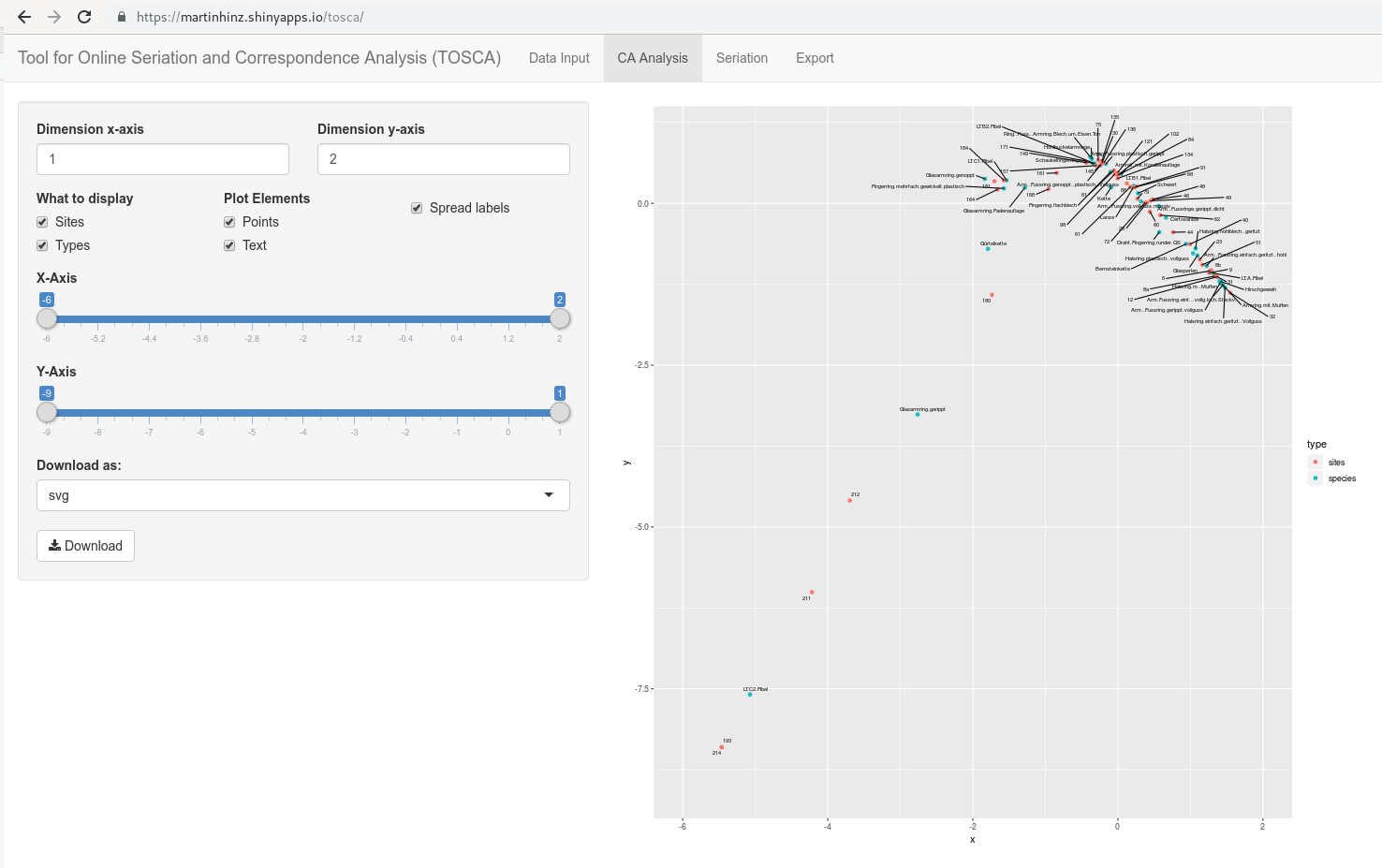
![](../images/12_session/tosca.png)
]

.pull-right[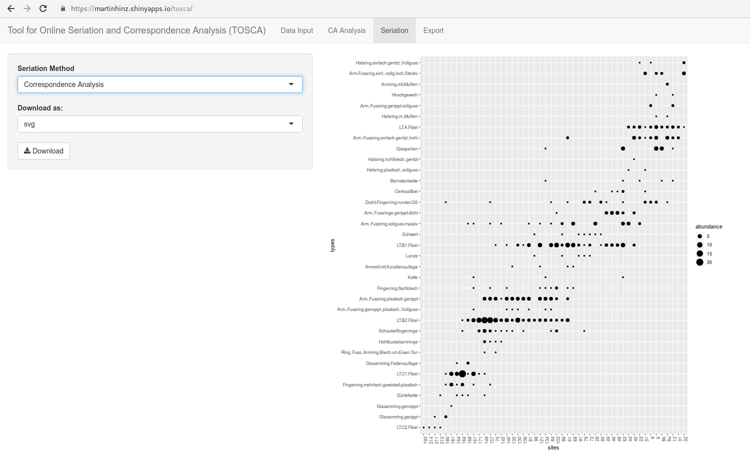
![](../images/12_session/tosca_seriation.png)
]

[http://tosca.archaeological.science](http://tosca.archaeological.science)
---

## Correspondence Analysis: Interpretation

### Guttman effect (horseshoe, parabola)

.pull-left[
In archaeology, this is often regarded as evidence of a temporal orientation.

The Guttman effect occurs when a process affects the data on multiple levels.

The largest influencing factor, given a longer runtime, is mostly the time, but:

This does not always have to be the case.

Check against other information necessary.
]

.pull-right[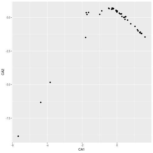
![](session_12_correspondence_analysis_files/figure-html/unnamed-chunk-31-1.png)
]